Conditional Addition In Google Sheets
Select your trigger from the Format cells if. Here are a few things you can do with an add-on that extends Google Sheets.
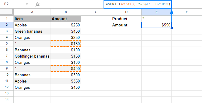
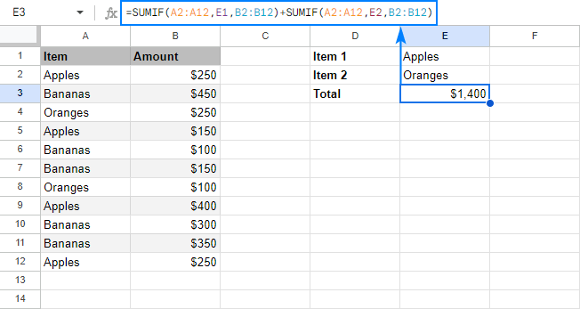 Sumif In Google Sheets With Formula Examples
Equivalent to the operator.

Conditional addition in google sheets. Returns the sum of values selected from a database table-like array or range using a SQL-like query. From the Format menu choose Conditional formatting. Change the Format cells if dropdown to Is equal to.
A suggestion box appears to help. Isbetween A21100 image 4. Select the range that you want formatted.
The steps to follow are. In the Apply to range box click the icon on the right for. Format Rules are the conditions based on which Google Sheets will apply conditional formatting on your selected data range.
2 hours agoIm using the conditional formatting in google sheets and Im encountering a problem in which every time I do any kind of action like copypaste the CF range changes and I end up with a whole mess of colored cells. For example you might say If cell B2 is. But there is a workaround which can help you to apply different icons based on condition similar to MS Excel icon sets.
Lets highlight the orders that are over 200 in Total sales and those that are under 100. Click Format Conditional Formatting from the menu. Google Sheets conditional formatting allows you to change the aspect of a cellthat is a cells background color or the style of the cells textbased on rules you set.
Add conditional formatting to the tables in Google sheet Conditional formatting is a data visualization technique that formats the cells text color text size cell background color etc if they meet certain conditions. You can read edit visualize and format data in Google Sheets spreadsheets using the. Once youve chosen your data click on the dropdown menu in the conditional formatting rules section and choose the condition you want to apply.
We can apply following two formula combinedly to achieve the similar feature. When you see your rule display in the right-hand sidebar click the rule. Select your style under Formatting style.
To do this click Add another rule. With this you can format the cells that you want to highlight. Format cells in Google Sheets by multiple conditions If the color scale seems too bright to you you can create several conditions under the Single color tab and specify a format for each condition separately.
There are three arguments in the Google Sheets If function. In addition to the above examples we can use the ISBETWEEN function in Google Sheets to write custom formula rules in conditional formatting. Returns a conditional count across a range.
MMULT matrix1 matrix2 We must apply the conditions in the matrix 1. In Google Sheets the If statement is entered by typing into a cell. You can use Conditional Formatting in Google Sheets to format a cell based on its value.
In Google Spreadsheet conditional formatting allows background and font formatting icon sets are not yet supported. Google Sheets makes your data pop with colorful charts and graphs. Here are the different types of Format Rules you can choose from the list.
You can use Conditional Formatting to highlight cells with the score less than 35 in red and with more than 80 in green. Click on the Format menu. Click Format Conditional Formatting.
There are three parts in the above conditional group-wise running total array formula in Google Sheets. So you can add more visual effects to your data table. Highlight the range of cells that you want to be eligible for conditional formatting.
Test Then_true and Otherwise-Value. All for free. Every rule you set is an ifthen statement.
Enter some example values in a few rows. Equivalent to the - operator. The syntax is if test then_true otherwise_value.
Built-in formulas pivot tables and conditional formatting options save time and simplify common spreadsheet tasks. To access the Custom Formulas in Google Sheets Conditional Formatting. This article explains how to use the Google Sheets If function.
For example to highlight the entire rows if the numbers in A2A are between 1 and 100 we can use the below rule. The first two parts form the matrix 1 and the third part forms the matrix 2. Navigate the dropdown menu to near the bottom and click Conditional formatting.
Start with a new spreadsheet and follow the steps below. How it works. Returns one number divided by another.
Add the Same Rule to Multiple Cell Ranges Select the cell range or any cell in the range for the first rule. Avr-gcc using repeated addition instead of MULU instructions. For example suppose you have a data set of students scores in a test as shown below.
 Sheets Conditional Formatting Based On Another Cell Learn The Truth About Sheets Conditional Social Media Calendar Template Google Sheets World Data
 Duration Formats In Google Sheets Elapsed Time Units Google Sheets Time Unit How To Apply
 Excel Sumif Function Formula Examples To Conditionally Sum Cells Microsoft Excel Formulas Excel Excel Calendar Template
 Copy Of Accomplishing Great Feats With Google Sheets Google Sheets Google Tricks Digital Organization
 How To Add Formulas Functions In Google Spreadsheets By Andrew Childress Dive Into This Beginners Guide To Ge Google Spreadsheet Google Sheets Google Tricks
 Google Maps Formulas For Google Sheets Digital Inspiration Google Sheets Google Maps Custom Google Map
 Illustration Of Custom Formula Based Condtional Formatting In Google Apps Google Sheets Google Apps How To Apply App
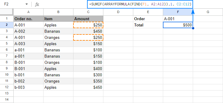 Sumif In Google Sheets With Formula Examples
 Google Sheets Bowling Scores Chart Review Distance Learning Google Sheets Bowling Bowling Tournament
 How To Create Conditional Formulas In Adobe Acrobat Financial Documents Syntax Formula
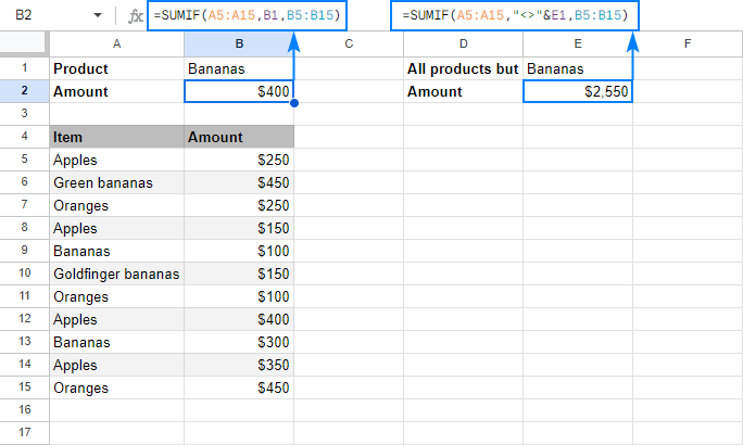
 Sumif In Google Sheets With Formula Examples
 The 7 Most Useful Google Sheets Formulas Google Spreadsheet Google Sheets Google Platform
 Sumif In Google Sheets With Formula Examples
 Google Sheets Sumif How To Use Sumif Formula Step By Step Tutorial Youtube
 How To Automatically Alternate Row Or Column Colors In Google Sheets Google Sheets Google Tricks Google Tools
 Adding Formulas In Google Sheets Google Sheets Useful Life Hacks Formula
 How To Automatically Alternate Row Or Column Colors In Google Sheets Google Sheets Google Drive Tips Google Education
Google Sheets Formulas For Analyzing Marketing Data Analyticalmarketer Io
 Sumif In Google Sheets With Formula Examples